The content of this page was originally posted on July 12, 2013. The HTML code was modified to be HTML5 compliant on July 12, 2013.

The interactive plot on this page is a Mathematica Computable Document Format file and requires the use of the free Wolfram CDF Player.

Directivity Pattern for an Acoustic Doublet (Bipole)

Two identical simple sources (monopoles) are separated by a distance of 2d and driven in phase comprises a sound source called an acoustics doublet or bipole.

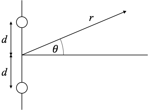
The resulting directivity pattern of the radiated sound depends on angle θ (which is measured from the plane bisecting the two sources), the separation distance between the two sources d and the frequency which is usually expressed in terms of the wavenumber k. The dimensionless quantity kd tells us the relative comparison of the wavelength of the sound and the separation of the sources. If kd≪1 then the sources are close together compared to a wavelength (small size doublet or low frequency) and the source looks like a simple monopole with double strength. When kd≫1 then the sources are far apart together compared to a wavelength (large size doublet or high frequency) and the directivity pattern has a large number of grating lobes, or angular directions where the sound radiates equally well.

The animation at right shows how the directivity pattern (drawn in 2-D) changes as the quantity kd varies from 0 to 5π and back to 0 again.

The interactive plot at right shows a 3-D rendering of the directivity pattern for the acoustic doublet. You will need to install the free CDF Player from Wolfram in order to view and interact with the plot.

The two small spheres in the plot show the orientation of the doublet sources. They are not to scale, and their positions do not adjust as you change kd. They are only shown to indicate the axis along which they lie, to help with the orientation of the directivity plot.

Moving the slider changes the value of kd from 0 to 5π. It may take a second or two for the plot to fully render after you moved the slider -- the applet is actually calculating and rendering the 3D image realtime, so you will get the best results if you move the slider in small increments and be patient while the new plot renders. Clicking on the [+] button at the right end of the slider bring up some additional controls as well as a window showing the actual value of kd. You can enter a number directly into this text window as well.

If you click somewhere in the plot window you should notice that the cursor changes (either a dot with an arrow circling around it or two arrows forming an ellipse). This allows you to rotate the 3D rendering so that you can view it from a different orientation. Just click in the plot window and drag your mouse to rotate the directivity pattern.