What are these graphs?
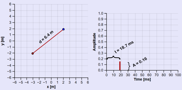
Start with 0 walls and compare the two graphs. The left shows a sound source (red) and a receiver (blue) in space. If the source makes an impulse (like a clap), the right graph shows what would be recorded by the receiver. There will be some time \( t \) before the pulse arrives, and it will have an amplitude \( A \) when it arrives. Both are determined by the distance \( d \) between source and receiver: \[A = \frac{1}{d} \quad,\quad t = \frac{d}{c}\]
Show Example
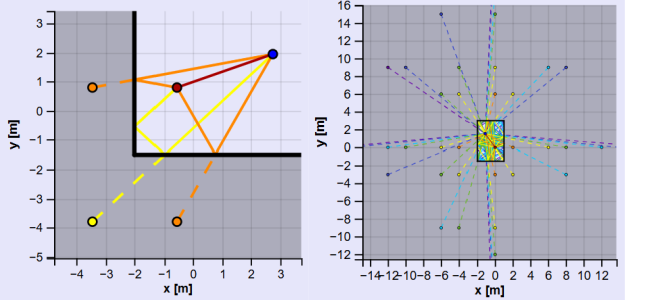
The colored lines on the left plot show the possible paths from the source to the receiver with the colors corresponding to the number of reflections. Hitting play shows expanding circles representing the wavefronts radiating from the source and image sources. The animation is played at \( \frac{1}{200} \) speed for visibility.
Show the Math
The distance between source and receiver \(d\) determines the time of arrival \(t\) via the speed of sound which is assumed to be \(c = 343 \ m/s\) \[t = \frac{d}{c}\]
The amplitude can be calculated using only the distance if we make a few assumptions. First, the source radiates outward in a perfect sphere (point-source) — we are only working with 2D here so it will be circle. Next, the distances involved are small enough that the drop in amplitude is only due to the wave spreading out (negligible atmospheric absorption). With these assumptions, the pressure radiated from a point-source is: \[p = \frac{j\omega\rho_0\hat{Q}e^{jkr}}{4\pi d}\]
We are going to be making our model with a perfect impulsive. It is infinitely loud over an infinitely short time. Because of this, it would not make sense to worry about any phase content, so let's look at just the amplitude: \[|p| = A = \frac{\omega\rho_0\hat{Q}}{4\pi d}\]
The instantaneous nature of the impulse makes the driving frequency \( \omega \) and source strength \( \hat{Q} \) necessarily constant, and it is reasonable to assume that the background density \(\rho_0\) is the same across the room. This leaves us with a simple proportionality: \[|p| \propto \frac{1}{d} ≡ A\] \[ A = \frac{1}{d} \]
With these two relations \(A = \frac{1}{d} \;,\; t = \frac{d}{c}\), we can calculate the pulse received using only the distance from source to receiver.
The Image Source:
Set the number of walls to 1 and there are now two paths to the receiver — a direct path and a reflected path. Hit play and compare the wavefronts with and without visibility behind the wall. The source reflected over the wall is called an image source. The wavefronts created by the source reflecting from the wall is identical to the one created by the image source.
Show Example
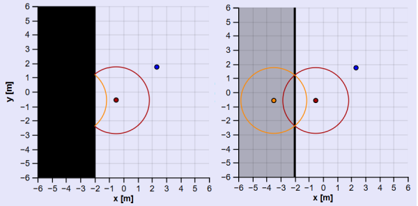
For this to work, we have to assume there is no scattering from the walls — they are perfectly smooth so we get specular reflections. We also have to assume that the wavefronts have a curvature large enough to be almost flat (quasi-planar) when hitting a wall. With these assumptions, we can treat the wave like a ray bouncing around the room.
We can use the image sources to find the paths from source to receiver. Start at the receiver and draw a straight line to the image source (shown as dashed lines). This gives the the last leg of the path and the intersection point with the wall. Repeat this process with a line back towards the previous image source until that is the original source.
Images of Images:
Set the number of walls to 2 and the max order to at least 2. We have the two reflected images, but there is now a third path which bounces off both walls. For this path, we need to reflect an image source over the other to get what's called a second order image source.
With more walls, there are more possible paths and corresponding images. If walls are parallel or the space is enclosed, there exist an infinite number of possible paths and image sources. Accounting for longer paths allows you to calculate a longer impulse response.
Show Example
A complex room can take immense computational power if a long impulse response is needed due to the immense number of possible image sources at high orders. This is compounded by the need to check whether each possible image source represents a valid path.
Valid Image Sources:
Reflecting every image source over each wall doesn't always create an image source representing a valid path from source to receiver. Each needs to be tested for a path tracing back to the source.
Let's look at the second order reflection for a scenario with two walls. For a typical 90° corner the two possible image sources land in the same place, but only one represents a valid path. The correct one is determined by the location of the receiver.
Here is a corner of 85° so you can see the two possible second order image sources. The left plot shows how (\( S_{21} \)) is the valid image source. Draw a line (yellow dashed) from it to the receiver (\( Rcv \)). From the wall intersection, draw a line (orange dashed) to (\( S_2 \)) because it was used to make (\( S_{21} \)). The path can be completed to the source (\( S \)) and all angles will obey the law of reflections.
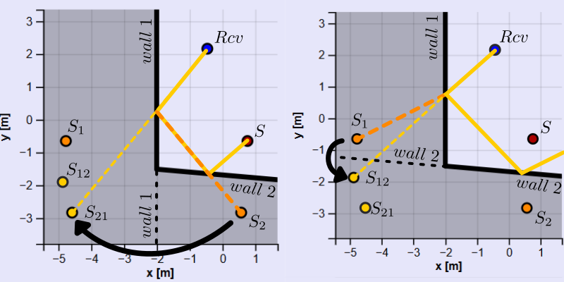
The right plot shows why \( S_{12} \) is an invalid source for the receiver position. After the first wall intersection, the line drawn to \( S_1 \) does not intersect wall 2. Without an intersection with wall 2, we know that it is not possible to get from the source to the receiver by hitting wall 2 before wall 1.
The solid yellow line was continued via the law of reflections just to show that it would not return to the source. \( S_{12} \) does not represent a valid image source and should not be included when calculating the impulse response. \( S_{21} \) would be the invalid image source if the receiver were on the other side of the line drawn from the corner through the source.
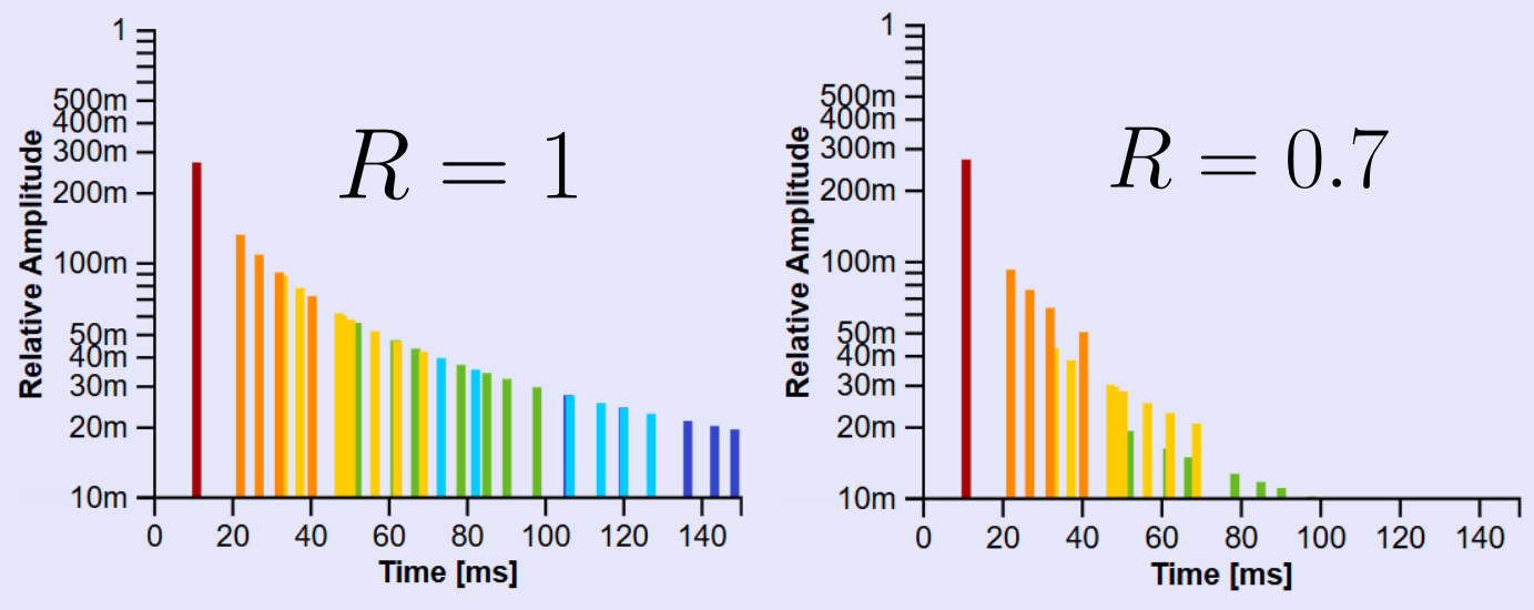
Wall Absorption:
If we make some simplifying assumptions, then we can calculate the amplitude of signals received while accounting for absorption by the walls. We will use the reflection coefficient \( R \) which is the ratio of amplitude before and after reflecting from a wall. \( R = 1 \) indicates total reflection while \( R = 0 \) indicates total absorption.
Assumptions to make this true
The reflection coefficient of a surface is typically not a single number, but a series of numbers corresponding to third-octave bands of frequencies. We are assuming that the excitation is a perfect impulse, so treating it as having frequency content would not make sense.
This model is assuming the wall to be perfectly smooth so there is no scattering (diffusion). Including diffusive reflections creates a far more accurate acoustical model of a room, but is far more mathematically complex.
It is assumed that the reflection from the walls is the same regardless of the angle of approach. This is true for planar waves but breaks down for spherical waves approaching at shallow angles. This model assumes that all reflections occur at a sufficient distance from the source that the wavefront is approximately planar.
The reflection coefficient \( R \) simply scales the amplitude for each reflection on the path. Assuming all walls are identical, the amplitude received from each image source is: \[A = R^n\frac{1}{d}\]
where \( n \) is the number of walls hit or the order of reflection, and \( d \) is the distance traveled.
Show Example
Impulse Response:
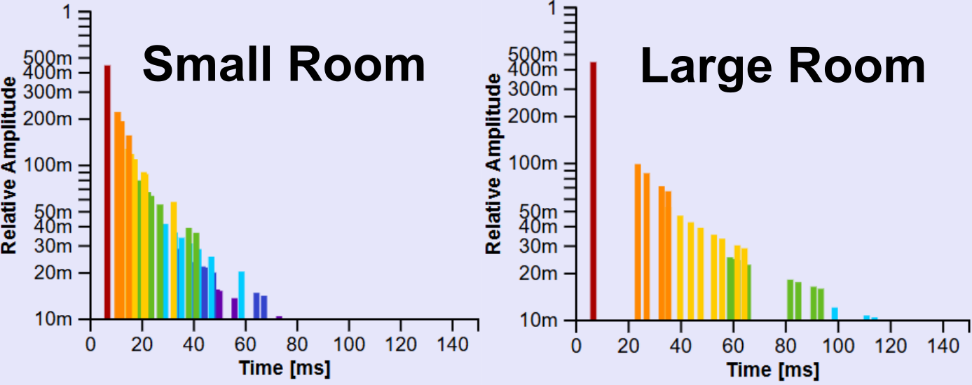
The plot on the right is an impulse response for the transfer from the source to the receiver. There are also many characteristics of the room in general that can be calculated using an impulse response, but let's look at it generally to gain insights into how well we might hear someone if they were speaking from the source location and we were listening from the receiver location.
Compare the same source and receiver locations for the 4 walled room and the "4-big" room. With speech, you want as many reflections as possible to reach within the first 50ms. These are known as early reflections. Reflections that arrive later than 50ms will be noise interfering with the next syllables spoken (late reflections). Reflections received about 100ms after the initial are perceived as an echo if they are preceded by a silent gap. Otherwise, reflections received this late contribute to the perceived reverberance of the room.
Show Example
What if the source is playing music? The quiet gaps between sounds is less critical than for speech, so the desirable early reflections is expanded to about 60ms. Much later reflections may even be good if you want a reverberant sound.
What does this tell us about how reverberant the room is? Reverberance is measured by turning off a source that had been playing for a while and measuring how long it takes for the sound in the room to decay by 60 dB. This is not the same as exciting the room with an impulse, so we can't directly tell the reverberance from the impulse response; However, we can still see the same trends in the impulse response. Look at the response after about 80ms for an idea of how reverberant a room might be.
Discussion Points:
- Place the source near a corner. What do you notice about the impulse response? What happens when you actually place a source (your phone playing music) in a corner?
- hint: The time-resolution of this impulse response is infinite. Pulses very close together will add in amplitude.
- Comparing the big and normal 4-walled room, how does the difference in impulse responses compare to your experience in large and small rooms?
- What changes if you switch the source and receiver?