Standing Longitudinal Sound Waves
The problem: using static graphs to depict standing waves
While teaching undergraduate physics at Kettering University for 16 years, I was often frustrated with the depiction of standing sound waves in pipes as it was presented in most elementary physics textbooks. Even textbooks specializing in wave phenomena were often not much better. Students are generally introduced to the concept of standing waves through a discussion of transverse standing waves on a string.
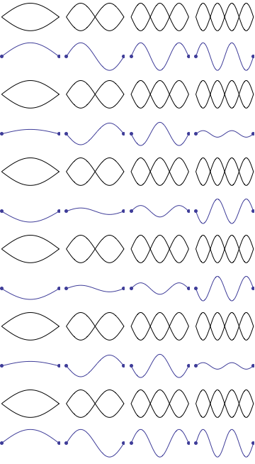 Static images of standing waves on a fixed-fixed string, like those shown at right, are more readily understood intuitively because the static "graphs" showing standing wave patterns correspond directly to the transverse displacment of the string, as depicted in the animation shown. As the string moves up and down the displacement fits into the envelope of the static graphs representing the standing wave patterns.
However, sound waves are longitudinal waves and the particle motion associated with a standing sound wave in a pipe is directed along the length of the pipe (back and forth along the pipe axis, or left and right horizontally for the images shown at right). It is a bit more difficult to imagine horizontal motion depicted by graphs that appear to show vertical displacement, and this is the problem I have with most textbook treatments of standing sound waves.
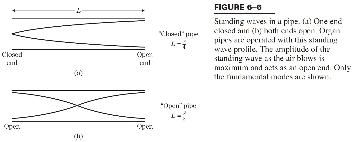 For example, the figure shown at right is from a specialized textbook[1] that I used for several years while teaching an upper level undergraduate physics of waves course to physics majors. The figure caption states that the figure shows "standing waves in a pipe" but does not indicate what quantity is being represented by this "standing wave profile." Is the plot showing displacement, or pressure, or something else? The caption mentions the "amplitude of the standing wave" but again does not define what that amplitude represents. The answer is that he curves in the figure represent the extremes of the horizontal particle displacement amplitude the acoustic particles in the gas medium as the standing wave oscillates through a complete cycle, but such an interpretation is not readily apparent from such a graph, and certainly not apparent from this figure caption.
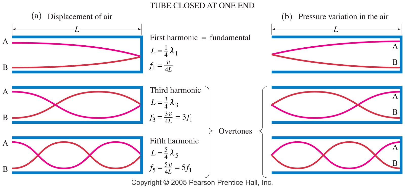 Other textbooks (like the Prentice Hall physics textbook from includes the figure at right) try to do better by showing two companion sets of graphs, one showing the displacement of air an the other for pressure associated with the sound wave. However, the displacement plots still don't clearly indicate that the displacement amplitude is for a longitudinal horizontal (left-to-right) motion of the air particles.
This problem of using static sinusoidal plots to represent longitudinal standing waves, and resulting student misunderstandings, was the subject of a Physics Education Research study several years ago.[2]
I created the animations below in an attempt to better explain the behavior of a standing sound wave in a pipe.
The solution: an animation to visualize particle motion and pressure for longitudinal sound waves.
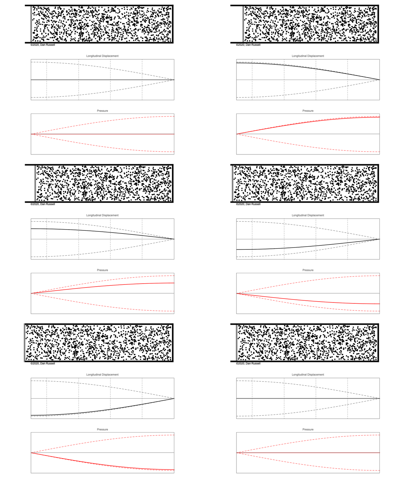
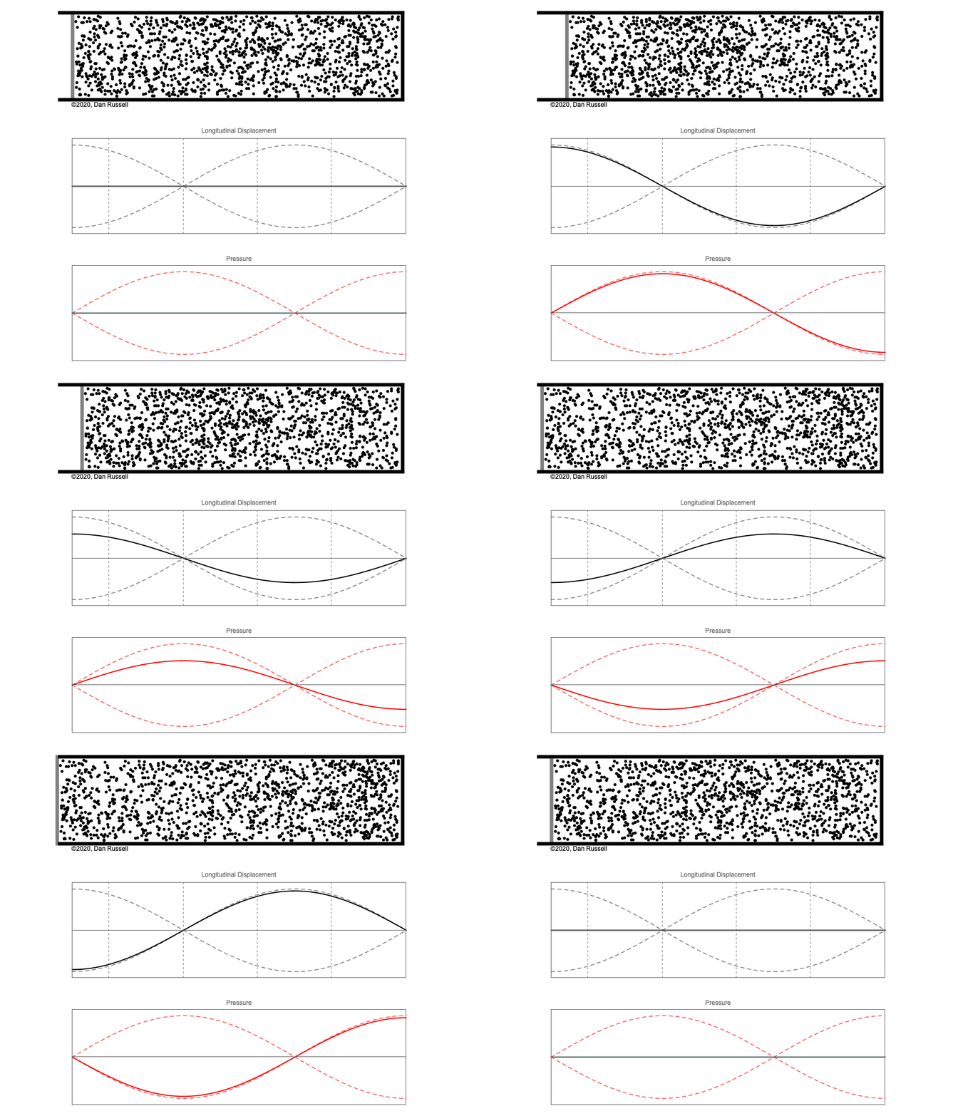
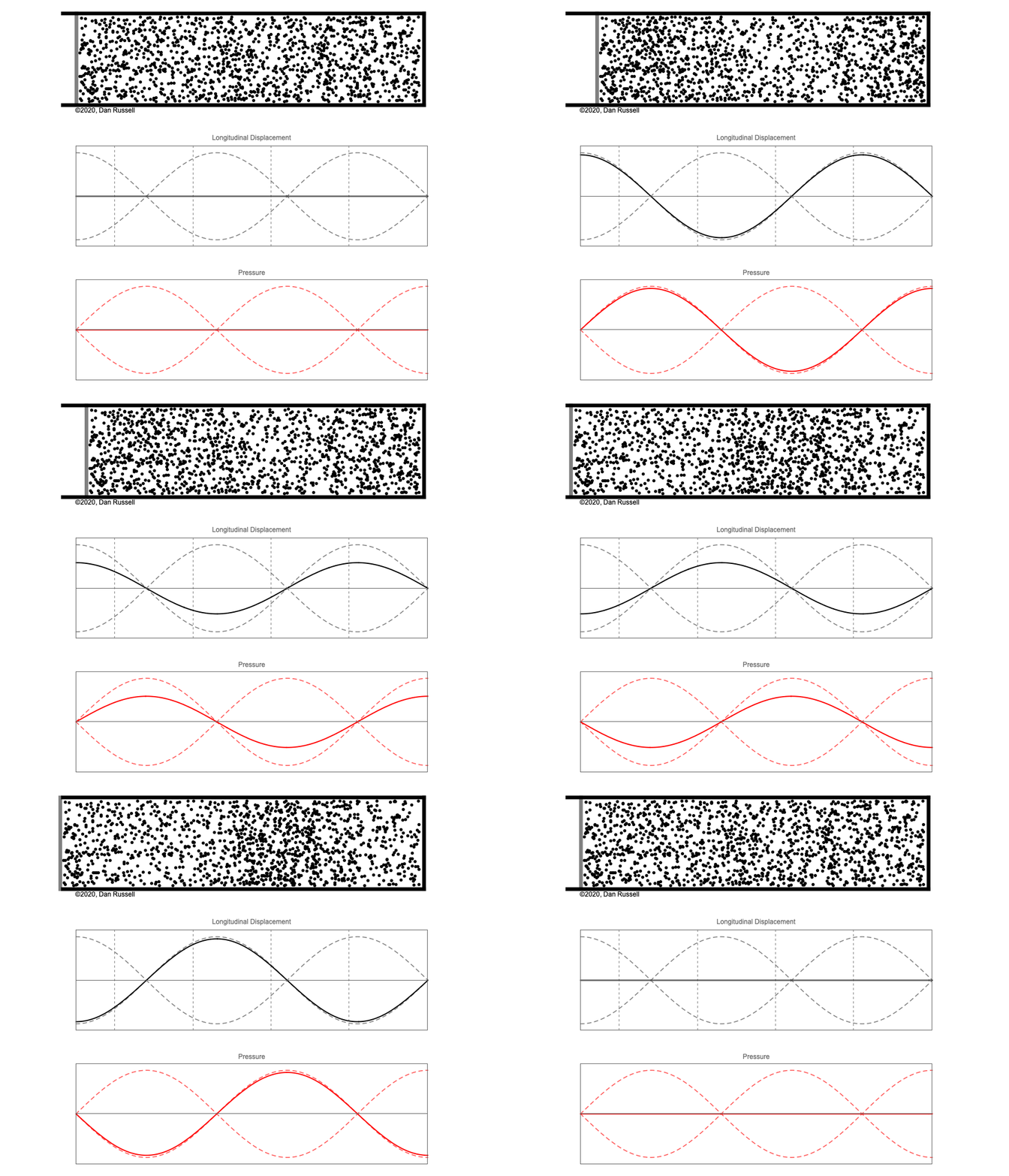
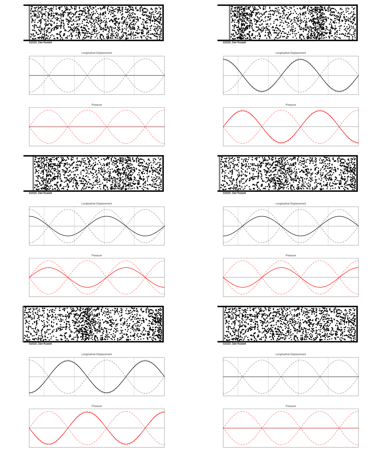
The particular examples of standing waves that I am illustrating here are standing sound waves in a pipe that is forced (by a moving piston or loudspeaker) at the left end and fixed, or closed, at the right end. (NOTE: this is the same standing behavior as for a pipe open at one end and closed at the other end.) The animations show the first five standing wave shapes (the first five harmonics) for the open-closed pipe.
Top plot: actual standing wave particle motion. The particles immediately to the right in front of the piston move with the piston as it oscillates back and forth. Elsewhere in the pipe, the particles oscillate back and forth, right and left, These particles are not all not all moving the same amount, and they are not all moving in the same direction at the same time; some are moving to the right while others are moving to the left. For each standing wave there will be at least one location where some of the particles do not move at all. These locations are displacement nodes, a location where the amplitude of the displacement always zero. Actually, for longitudinal sound waves in a pipe, a node is a plane that extends across the entire cross-section of the pipe. The particles on either side of a node move in opposite directions, alternately inward toward the node or outward away from the node. As the particles move toward the node, they become closer together and the local particle density at the node location increases (this would represent a compression). As the particles move outward away from the node the local particle density at the node location decreases (a rarefaction).
The closed end of the pipe acts as a displacement node; the particles cannot move beyond the rigid end, so the displacement is zero at the closed end. The piston face acts as a displacement antinode; the particles move with maximum displacement amplitude.
Middle graph: longitudinal particle displacement. The middle graph for each animation shows a graph representing the horizontal displacement of the air particles in the standing wave. When the graph is a horizontal line at zero all of the particles are at their equilibrium positions. Regions where the graph becomes positive represent regions where the particles are displaced from their equilibrium locations toward the right, in the positive \( x \)-direction. Regions where the graph becomes negative represent regions where the particles are displaced from their equilibrium positions toward the left, in the negative \( x \)direction. Locations where the particle displacement graph is always zero correspond to the to the displacement nodes.
Bottom graph: pressure variation. The bottom animation shows a graph representing the pressure variation associated with this standing sound wave. When the local density of the particles increases above the ambient value, the pressure variation is positive; this occurs when the particles are moving inward toward a displacement node location. When the local density of the particles decreases below the ambient value, the pressure variation is negative; this occurs when the particles move outward away from a displacement node location. If you compare the three animations, you'll notice that the pressure nodes (locations where the pressure is always zero) coincide with the displacement antinodes, there the local particle density does not change as the particles move back and forth together.