The Struck Fixed-Fixed String

The problem of the struck string is very similar to the problem of the Plucked String, in that there are two types of conditions which must be considered. The Boundary Conditions (ie, the values of displacement, velocity, and force at the each end of the string) determine the possible allowed mode shapes with which the string may vibrate at one of its natural frequencies. The Initial Conditions (the initial displacement and velocity of the entire string at time \(t=0\)) determine which of the possible allowed mode shapes actually participate in the ensuing motion, and with what amplitudes.

For a string which is fixed at both ends, the boundary conditions at each end require that the displacement of the string must always be zero. This results in mode shapes for which the transverse displacement at any point along the string depends on a sine function, $$ \sin\Big(\frac{n\pi}{L}x\Big)\ , $$ where \(L\) is the length of the string, and \(n\) is an integer. The animation at right shows the first four allowed mode shapes for a fixed-fixed string. The number of "humps" (antinodes) corresponds to the value of \(n\). After applying the boundary conditions, the complete expression for the transverse displacement of the string, as a function of time and postion along the string's length, is $$ y(x,t) = \sum_{n=1}^N \big [A_n\cos(\omega_n t) + B_n\sin(\omega_n t)\big ] \sin\Big(\frac{n\pi}{L}x\Big) $$ where \(\omega_n\) is the natural frequency of the \(n\)^th mode, and the coefficients \(A_n\) and \(B_n\) are determined from the initial displacement and velocity of the string, respectively. The string has a linear density \(\rho_L\) [kg/m] and is stretched to a tension \(T\); transverse waves travel along the string with a speed \(c=\sqrt{T/\rho_L}\). The natural frequencies corresponding to the allowed mode shapes depend on the wave speed and the string length, $$ \omega_n = 2\pi\, \frac{n c}{2 L} \ .$$ The natural frequencies will be higher if the string is shorter, or if the tension is higher, or if the density is lower. The natural (or allowed) frequencies are integer multiples of the fundamental (\(n=1\)) frequency.

Initial Conditions for the Struck String

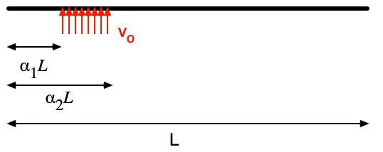The actual interaction between the piano hammer and string is a very complicated one, but we can get a rough approximation by using a crude model that assumes the entire string is initially at rest, with an initial velocity imparted to the string over a short segment of the string, as illustrated at right. The Fourier Coefficients, \(A_n\) and \(B_n\) are found from the initial displacement and velocity profiles of the string, $$ A_n = \frac{2}{L}\int_0^L y(x,0) \sin\Big(\frac{n\pi}{L}x\Big) \, dx \qquad \hbox{and} \qquad B_n = \frac{2}{\omega_n L}\int_0^L u(x,0) \sin\Big(\frac{n\pi}{L}x\Big) \, dx \ . $$ Since the struck string is initially at rest at its equilibrium position, all of the \(A_n=0\). The \(B_n\) depend on the details of the initial velocity.

As a first approximation, let's assume a uniform velocity \(v_o\) between \(\alpha_1 L\) and \(\alpha_2 L\) and zero elsewhere. From the integral expressions, we get $$ B_n = \frac{2 v_o L}{c (n\pi)^2} \Big(\cos(\alpha_1 n \pi) - \cos(\alpha_2 n \pi)\Big) $$ and the resulting transverse displacement of all points on the string as a function of time obeys $$y(x,t) = \sum_{n=1}^N B_n \sin\Big(\frac{n\pi}{L}x\Big)\sin\Big(2\pi\frac{n c}{2L} t\Big) \ . $$ The animation at right shows what how this sum of Fourier components builds up to represent what the string looks like at a fixed time very shortly after the hammer has struck the string and given a uniform velocity to a short segment (the summation in the equation is plotted as a function of x for a small but fixed value of time).

A slightly more realistic result may be obtained by letting the initial velocity profile take the shape of a half-cycle sine function, as shown at left. The math required to solve the integral expression for the \(B_n\) is more difficult, but the integrals may be solved with a numerical method.

The animation at right shows how the Fourier components build up for this improved model of the struck string, plotted as a function of x for the same fixed time. The differences between the two models are small; the improved version results in slightly narrower pulse.
I am constantly amazed that a Fourier sum of sine functions, with the right amplitudes and frequencies, can add up to a pattern like this!

Motion of the Struck String (after being struck)

The motion of the struck string is obtained by making a sequence of plots of the expression for the transverse displacement as a function of x for increasing values of time. This is illustrated in the animation below. After the hammer blow, the portion of the string with an initial velocity moves upward, pulling the adjacent string with it, and a pulse begins to widen left and right from the impact point. The left going edge reaches the near fixed end and reflects inverted, effectively canceling the displacement. As a result, a narrow "bump" travels to the right toward the far end of the string, where it reflects (inverted) and returns. One complete cycle occurs at the fundamental frequency of the string -- on the middle C string of a piano, this pulse will race down and back 262 times every second.

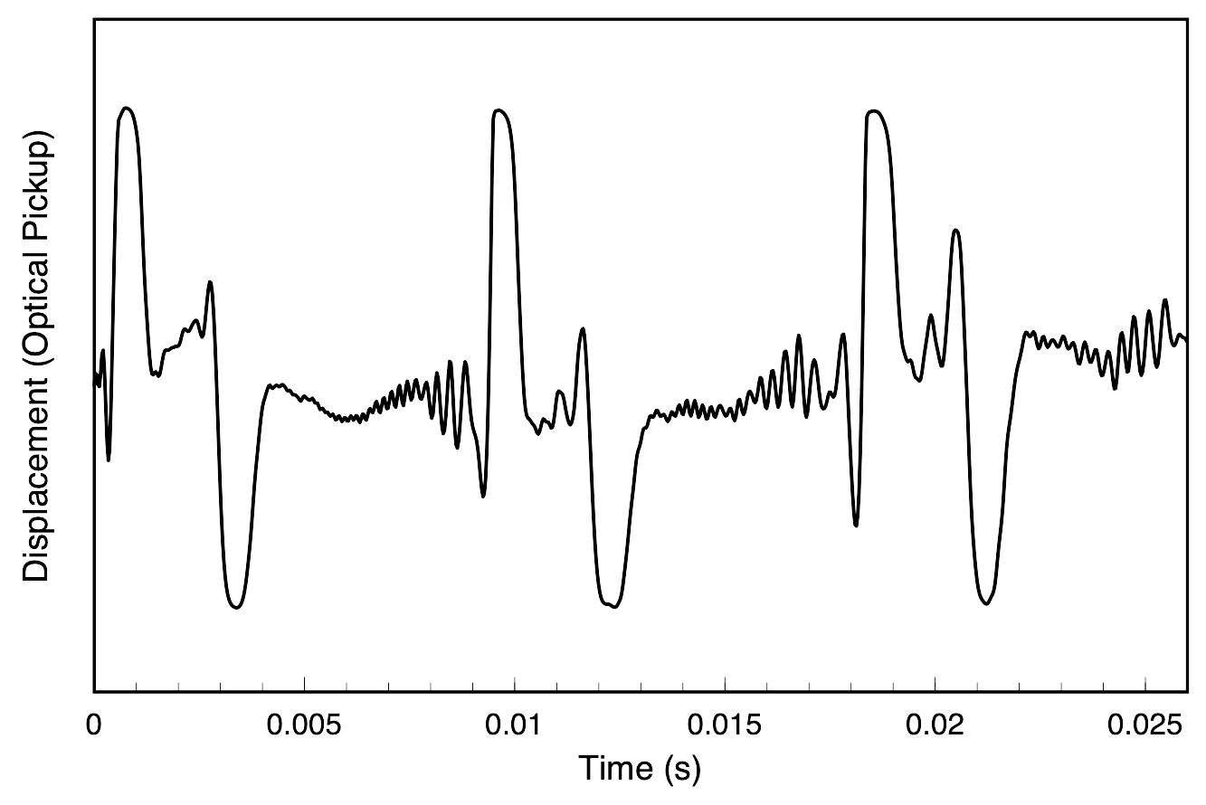
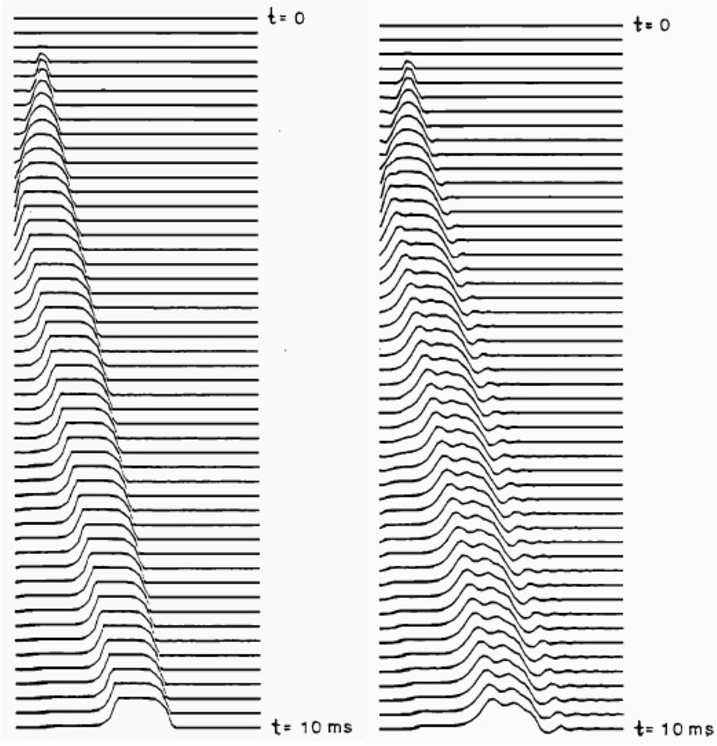The actual interaction between hammer and string in a piano is much more complicated -- the hammer is physically thrown back by the string as the reflection from the near end returns and pushes the hammer away, which generates a new set of pulses. However, the fact that the simple crude model shown here correctly captures the essential physics may be seen by comparing to the waterfall plots in the figure at right.^[4] The traces on the left show a more complicated model of the struck string and a more realistic velocity excitation; the plot on the right shows measured data for the transverse displacement of a piano string after being struck. The measured data shows some ripples which are due to dispersion; the stiffness of the copper-wound steel piano string causes higher frequency components to travel with a faster speed than lower frequencies, and the initial pulse shape begins to distort as it travels down the string. But, the general nature of the travelign pulse created by a hammer strike is represented by the simple model in my animation above.

If the string is struck at its midpoint, then as initial pulse widens, it will reach the right and left ends at the same time, and the resulting string motion will look as shown at right. Dr. Paul Cruickshank at the University of St Andrews School of Physics & Astronomy made the following high speed videos which show a real (elastic) string behaving pretty much exactly as my simple model predicts.

Motion of a Specific Point on a Plucked String.

Predicting the time behavior of a specific location on the string is as simple as plotting the transverse displacement equation as a function of time, for a fixed value of \(x\). The animation below illustrates what this time signal would look like as the string is vibrating -- the time history on the right shows the position, as a function of time of the dot near the left end of the plucked string. The point actually sits still, at rest (but below its equilibrium position), until the wave envelope reflects from the other end and then the point quickly jumps up and back down again.

This theoretical prediction is also backed up by experimental data. The plot at right shows the time signal measured by an optical photogate transducer that measures the postion of a point on the string; this data was recorded for a guitar string struck by a piano hammer at the far end of the string. The measured data has many noticeable ripples just before the big jumps -- these ripples are evidence of dispersion due to the stiffness of the string, which causes the speed of waves on the string to become dependent on frequency.