The content of this page was originally posted on January 23, 2017.
Phase Between Pressure and Particle Velocity (Plane Waves)
When discussing the behavior of longitudinal plane waves (i.e., sound waves air), the following statements are often made regarding the relative phase between the pressure and the fluid particle velocity[1]
the pressure and particle velocity are in-phase for a forward traveling (right going) wave,
but the pressure and particle velocity have opposite phase for a backward traveling (left going) wave.
Mathematically this is observed the presence of a negative sign for the left going part of the wave expression. But conceptually, this can be a bit tricky to understand.
EQUATIONS?
Right Going (Forward Traveling) Wave
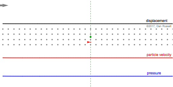
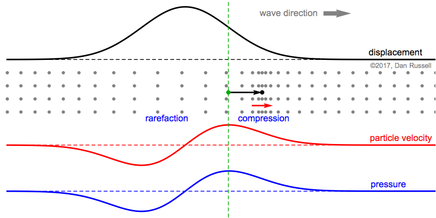
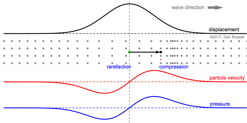
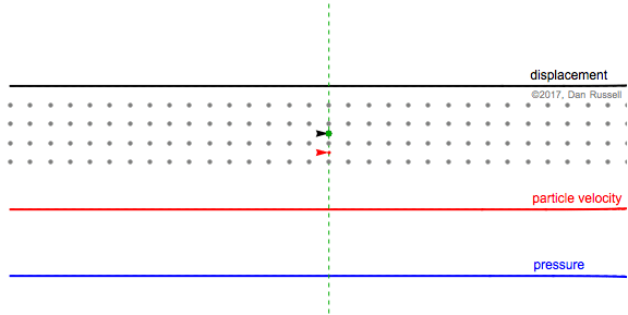
This animation shows a Gaussian pulse wave signal traveling in the positive (forward) direction, from left to right. The particle velocity and pressure are in-phase; positive velocity (moving right) occurs when pressure is positive (compression).
The gray dots represents the motion of the fluid particles in the medium, and as the wave travels from left to right, the particles are temporarily displaced to the right (in the positive direction) from their equilibrium postions, returning to equilibrium after the wave has passed.
The black plot and arrow represent the horizontal displacement of the fluid particle, originally at the green equilibrium postion, as the wave passes by. A large vertical value for the plot indicates a large positive horizontal displacement (to the right) from equilibrium.
The red arrow and plot represent the particle velocity. When the particles are moving to the right (in the positive direction), the velocity is positive and the arrow points to the right. When the particles are moving to the left (in the negative direction, back toward equilibrium) the velocity is negative and the arrow points to the left.
The blue plot and words represent the pressure. As the wave travels to the right, and the particles begin to be displaced in the positive direction (to the right) by different amounts, the particles at the leading edge of the wave are bunched together (compression) and the pressure is positive. As the wave passes, and the particles begin to move left (retuning to their equilibrium positions), the particles are more spread out (rarefaction) and the pressure is negative.
The first still frame at right shows that the particle (whose equilibrium location is identified by the green dot and dashed line) is being displaced in the positive direction, as evidenced by the black arrow to the right. At this instant, the particle is moving to the right with a maximum velocity (the red arrow points to the right, and the value of the particle velocity plot is a maximum (at the green equilibrium location). The neighboring particles (before and after the green equilibrium position) have been displaced to the right, and are now bunched together; so the pressure associated with the green equilibrium point location is a maximum.
The second still frame represents the time at which the particle (originally at the green equilibrium location) has reached its maximum displacement. At this instant, the particle velocity is zero. Also, the spacing between the displaced particle (originally at the green dot, but now displaced to the right tp the black dot at the tip of the arrow) and its displaced neighbors is the same value as when the particles were all at their equilibrium locations, so the pressure is zero.
The third still frame represents the time at which the particle (originally at the green equilibrium location) is still displaced in the positive direction (black arrow still points to the right), but the particle is moving to the left with a negative velocity as it returns to its equilibrium position. The particle is now further away from its neighbors than the equilibrium spacing (rarefaction), so the pressure is negative.
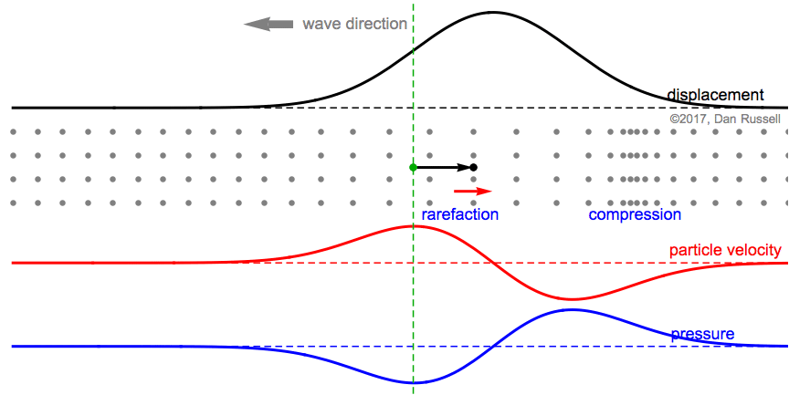
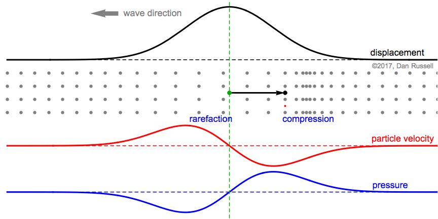
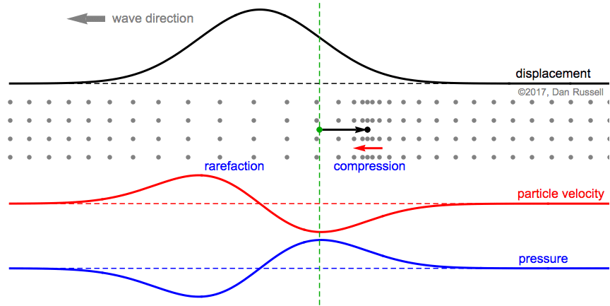
Left Going (Backward Traveling) Wave
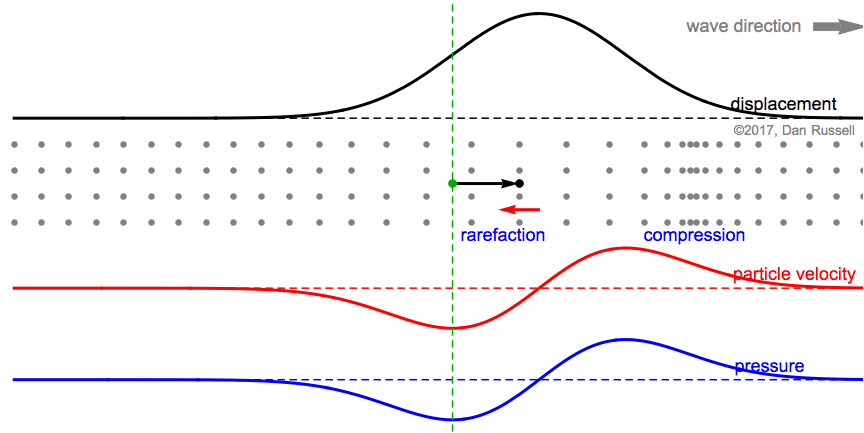
This animation shows the same postive Guassian wave pulse as above, except that now the wave pulse is traveling from right to left in the negative direction. The particle velocity and pressure are now opposite-phase; positive velocity (moving right) occurs when pressure is negative (rarefaction).
As the wave travels from right to left, the Gray particles are temporarily displaced to the right (in the positive direction) from their equilibrium postions.
The black plot and arrow represent the horizontal displacement of the the fluid particle, originally at the equilibrium location indicated by the green dot as the wave passes by. A large vertical value for the plot corresponds to a large positive horizontal displacement (to the right) from equilibrium.
The red arrow and plot represent the particle velocity. When the particles are moving to the right (in the positive direction), the velocity is positive and the arrow points to the right. When the particles are moving to the left (in the negative direction) the velocity is negative and the arrow points to the left.
The blue plot represents the pressure, with positive pressure corresponding to the region of compression where the particles are bunched together, and negative pressure corresponding to the region of rarefaction where the particles are spread apart. As this Gaussian wave pulse travels from right to left in the negative direction, the particles are first displaced in the positive horizontal direction (to the right), the particles at the leading edge of the wave become more spread out (rarefaction) and the pressure is negative. As the wave passes, and the particles begin to move left toward equilibrium, the particles become bunched together (compression) and the pressure is positive.
The first still frame at right shows occurs when the particle (whose equilibrium location is identified by the green dot and dashed line) is undergoing a displacement to the right, in the positive direction, as evidenced by the black arrow to the right. At this instant, the particle is moving to the right with a maximum velocity so that the red arrow points to the right, and the value of the particle velocity plot (at the green equilibrium location) is a maximum. The neighboring particles have been also displaced to the right, but are now spread apart from each other (rarefaction), so the pressure associated with the green equilibrium point location is negative.
The second still frame represents the time at which the particle (originally at the green equilibrium location) has reached its maximum positive displacement to the right. At this instant, the particle velocity is zero. Also, the spacing between the displaced particle (originally at the green dot, but now displaced to the right tp the black dot at the tip of the arrow) and its displaced neighbors is the same value as when the particles were all at their equilibrium locations, so the pressure is zero.
The third still frame represents the time at which the particle (originally at the green equilibrium location) is still displaced in the positive direction (black arrow still points to the right), but the particle is moving to the left with a negative velocity as it returns to its equilibrium position. The particle is now closer to its neighbors than the equilibrium spacing was (compression), so the pressure is positive.
References
David T. Blackstock, Fundamentals of Physical Acoustics (John Wiley & Sons, Inc., 2000), pg. 48.